

Tersa EDA

RF example

500 MHz low-pass filter simulation example

Explore a 500 MHz RF low-pass filter with its schematic, S11 and S21 plots, insertion loss, return loss, and component tuning in Tersa EDA.

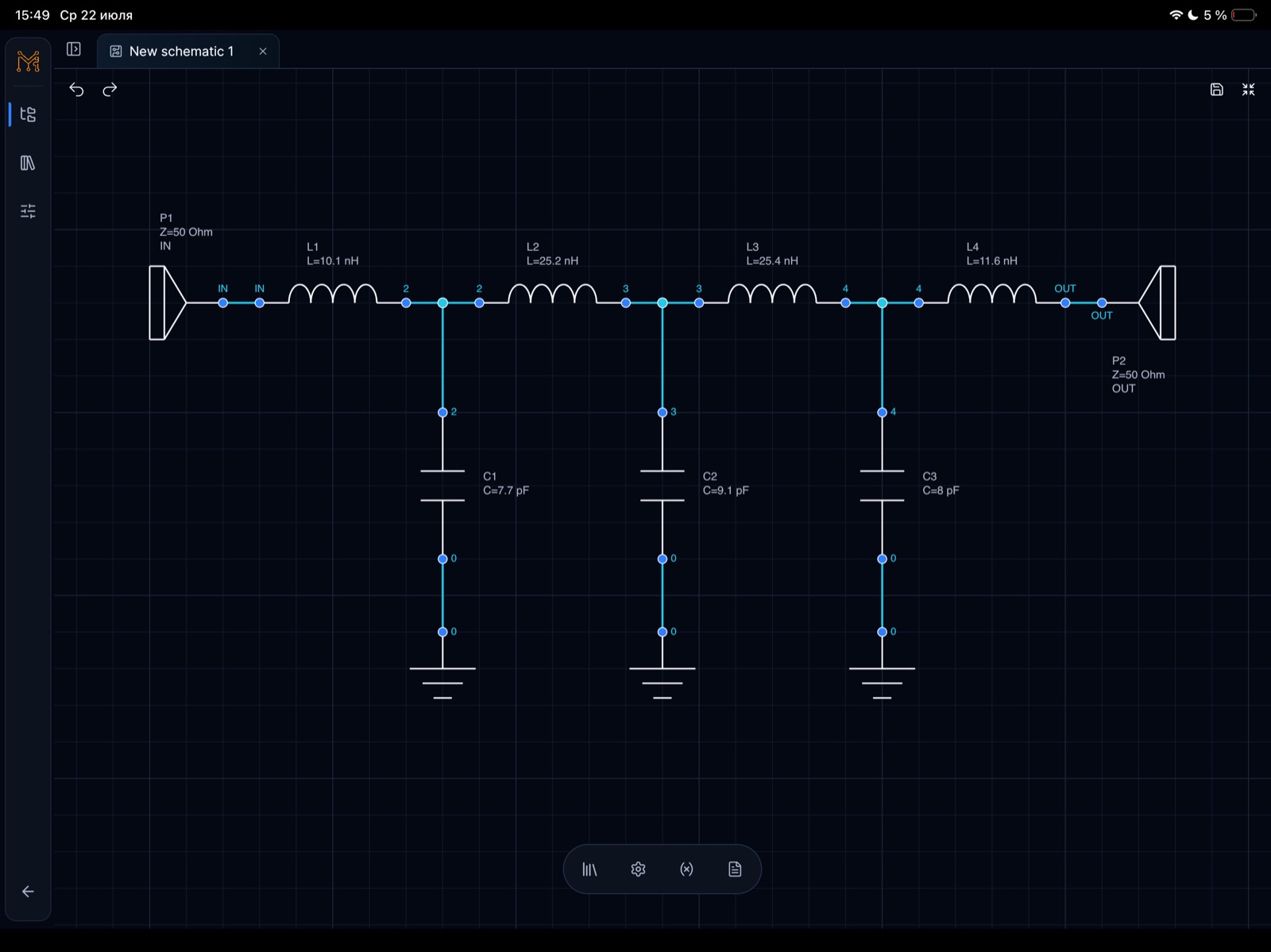
500 MHz low-pass filter schematic opened in the Tersa EDA workspace on iPad
Example
500 MHz LPF
Domain
RF filter design
Measurements
S11 / S21
Workflow
schematic -> plot -> tune

01

What this RF example demonstrates

This 500 MHz low-pass filter example follows the complete circuit workflow: build the ladder network, define 50 ohm ports, run an S-parameter analysis, inspect the passband and stopband, then tune the reactive components.

  • Schematic capture for an RF low-pass filter
  • Frequency-domain response around the cutoff region
  • Insertion loss and return loss inspection
  • Component-value tuning without leaving the workspace

02

Reading the filter response

S21 shows transmission through the filter and makes the cutoff transition visible. S11 and S22 show how well the source and load ports are matched across frequency, while markers help compare exact values at the design target.

  • Check passband insertion loss
  • Locate the cutoff transition
  • Inspect input and output return loss
  • Compare traces from DC to 1 GHz

03

How Tersa EDA fits the workflow

Tersa is positioned as a lightweight RF and analog tuning workspace: draw or open a circuit, choose analysis, inspect plots, place markers, and tune values quickly.

  • Designed for tablet and desktop use
  • Focused on RF/analog tuning rather than PCB layout
  • Connected to Smith chart and measurement views
  • Suitable for demo-driven beta onboarding

FAQ

Is this a real Tersa EDA example?

Yes. The page uses product screenshots from the Tersa EDA interface and focuses on a 500 MHz low-pass filter workflow.

What does the example measure?

It is positioned around S-parameter response, insertion loss, return loss, and tuning behavior around the filter target.

Why simulate beyond 500 MHz?

Sweeping beyond the target frequency makes the transition and stopband visible, so component changes can be evaluated against both passband and rejection goals.